Kalman Filter- Lidar+Radar Sensorfusion with EKF
동일/싱글 pedestrian에 대한 Lidar+Radar 센서퓨전
2021-09-15 10:10
Lidar+Radar Sensorfusion with Extended Kalman Filter
Author: SungwookLE
DATE: ‘21.9/14
Comment: Radar+Lidar Sensor Fusion Project on Udacity(Self-Driving Car Engineer Nanodegree Program)
GIT REPO: My implementation
In this project you will utilize a kalman filter to estimate the state of a moving object(pedestrian) of interest with noisy lidar and radar measurements. Passing the project requires obtaining RMSE values that are lower than the tolerance outlined in the project rubric.
Assumption: Single and Same Target Information would be continuously received
1. Pre-requires
- Simulator: Term 2 Simulator which can be downloaded here
- Communication Protocol Between Simulator and Your program: This repository includes two files that can be used to set up and install uWebSocketIO for either Linux or Mac systems. Please see the uWebSocketIO Starter Guide page in the classroom within the EKF Project lesson for the required version and installation scripts.
2. Introduction
프로젝트의 In/Out에 대해 설명하고 Sensor Fusion 로직 flow를 설명한다.
2-1. In/Out Description
1) INPUT: values provided by the simulator to the c++ program
- [“sensor_measurement”] => the measurement that the simulator observed (either lidar or radar)
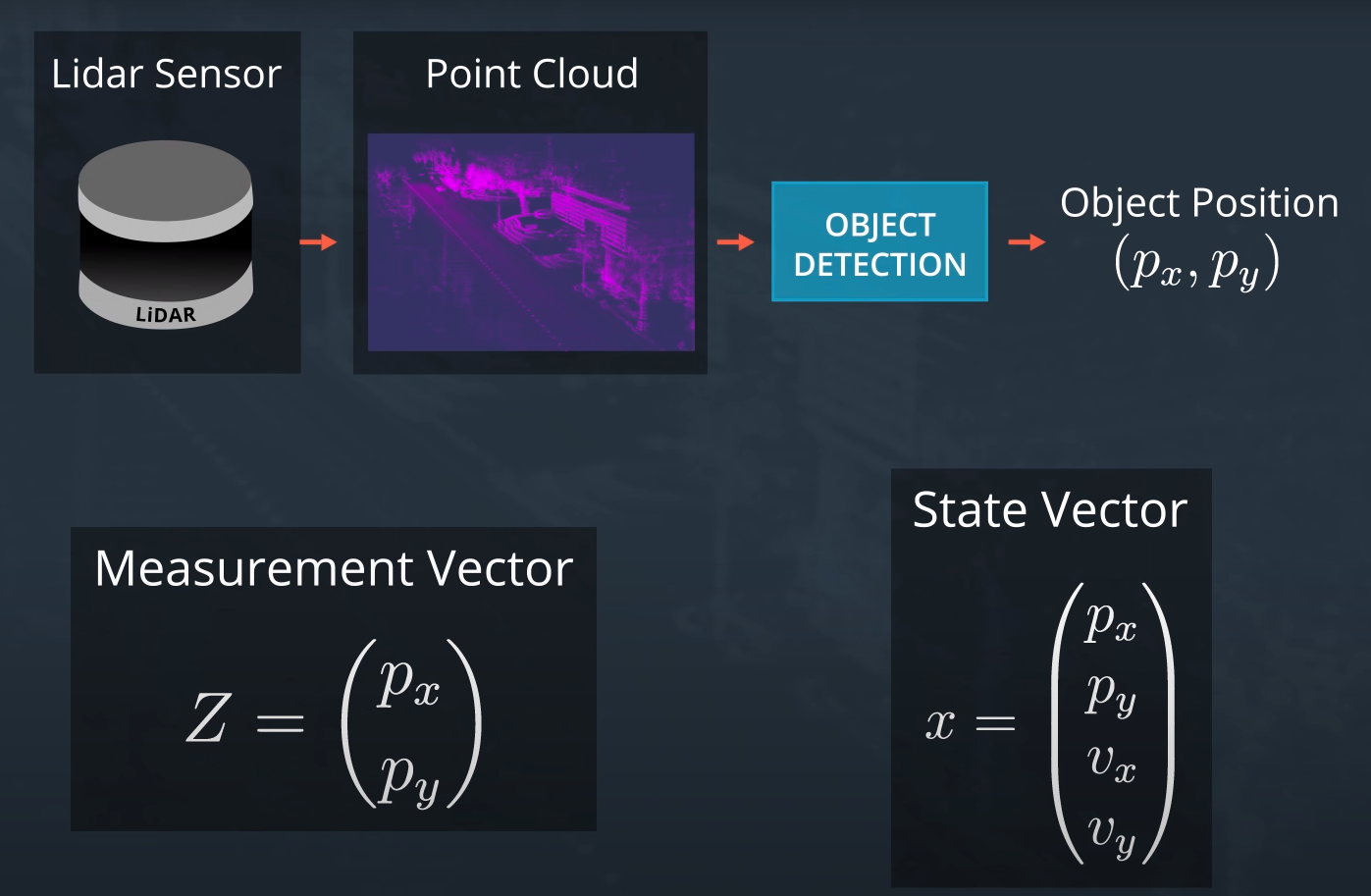
- 1-1) Lidar Data
- 1-2) Radar Data
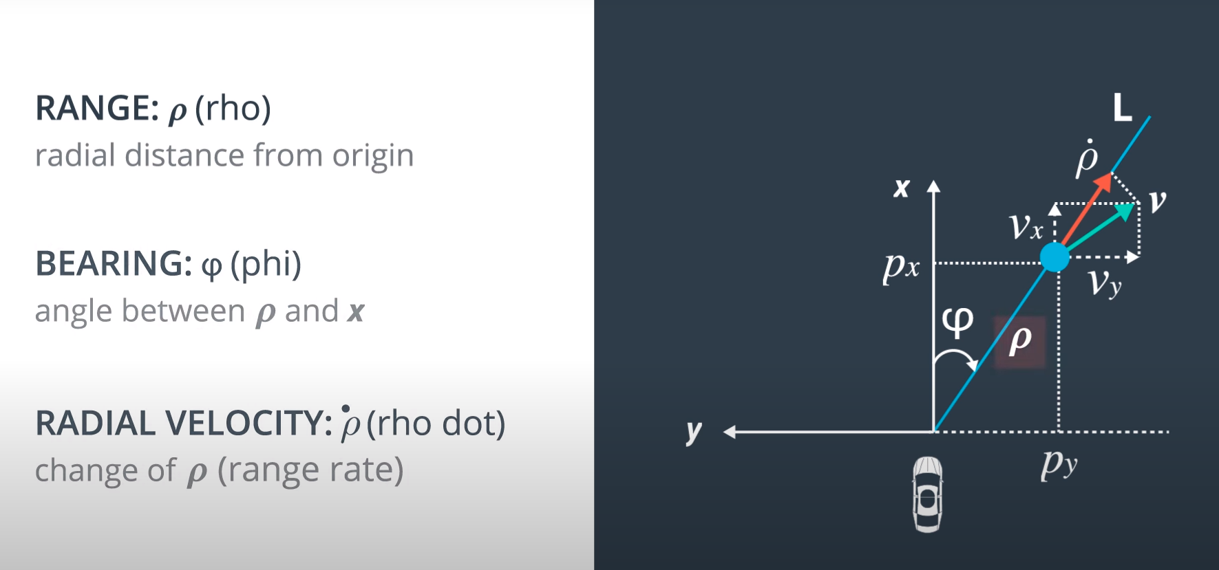
레이더 데이터는radial velocity, radial distance, radial degree를 제공하므로 극좌표계를 수직좌표계로 변환하는 과정에서non-linearity가 발생한다. 이 수식을 선형화해서 풀어야하고, 이런 방식으로 접근하는 것을 Extended Kalman Filter라고 한다.- 1-2-1) Linearlization
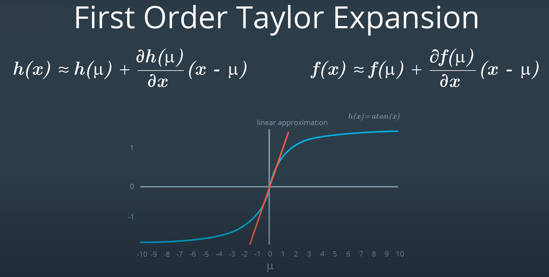
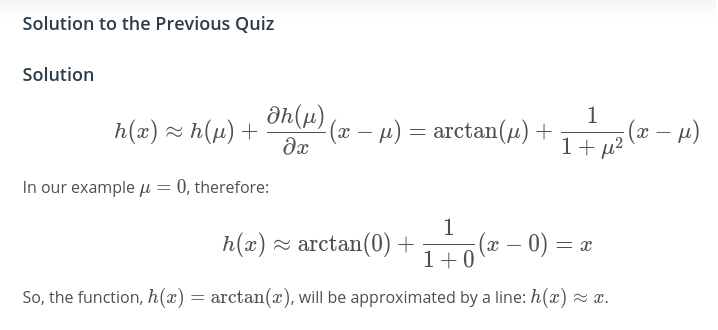
보이다시피, 현재 시점의 $\mu$값을 기준으로 선형화를 해야한다. :perturbation.
현재 시점이 0이라고 했을 때 h(x) = arctan(x) 의 테일러 1차 전개를 이용한 선형화 예시.
- 1-2-1) Linearlization
2) OUTPUT: values provided by the c++ program to the simulator
- [“estimate_x”] <= kalman filter estimated position x
- [“estimate_y”] <= kalman filter estimated position y
- [“rmse_x”]
- [“rmse_y”]
- [“rmse_vx”]
- [“rmse_vy”]
2-2. Sensor Fusion Flow
-
The car will receive another sensor measurement after a time period Δt. The algorithm then does another predict and update step.
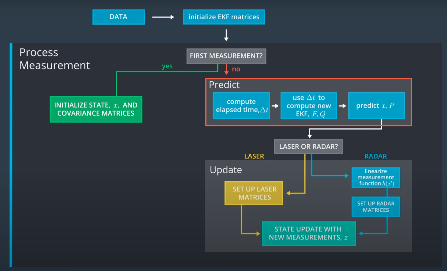
-
Lidar and Radar Sensor Fusion Flow in Kalman Filter 서로 다른 좌표계를 갖는 센서 데이터: Lidar(L)와 Radar(R) 를 받음에 따라 그에 맞는 칼만 업데이트(
update correctness)를 해주면 되고, 업데이트 된 값을 기준으로 매스탭마다prediction을 수행한다.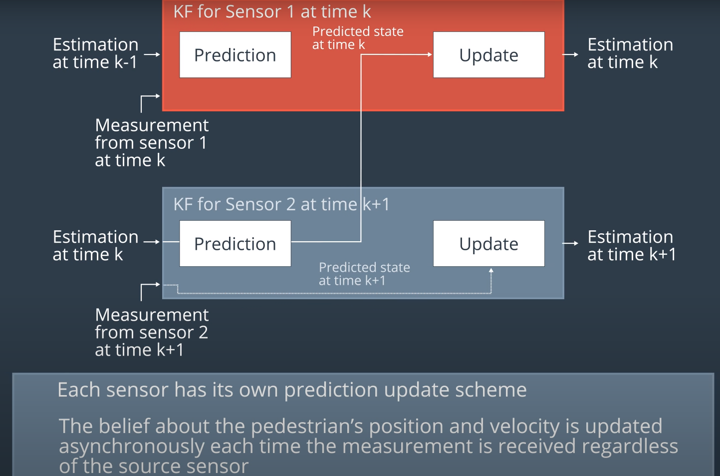
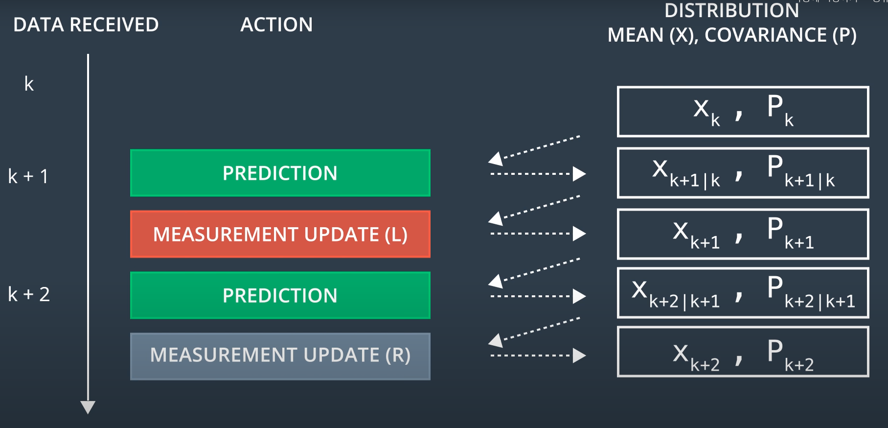
위 그림과 달리 Lidar와 Radar가 동시에 수신된다면, Update를 2번 해주면 된다. 무얼 먼저 update 과정을 거칠 것인지는 상관 없음. -
Radar 데이터의 경우
radial velocity, radial distance, radial degree가 출력되므로 이를 직교 좌표계로 바꾸는 과정에서 비선형 수식이 등장한다. 이를 해결하기 위해Extended Kalman Filter를 이용해야 하고EKF의 수식은 Linear Kalman Filter와 정확히 똑같지만, F와 H를 자코비안(테일러 1차) 선형화된 매트릭스로 대체하여 사용하는 것에 차이가 있다.
-
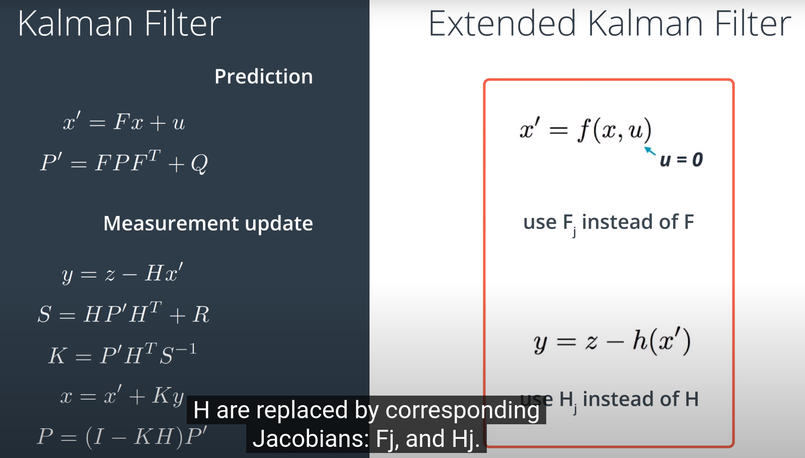
Extended Kalman Filter Equations Although the mathematical proof is somewhat complex, it turns out that the Kalman filter equations and extended Kalman filter equations are very similar. The main differences are:
- the F matrix will be replaced by $F_j$ when calculating
P'. - the H matrix in the Kalman filter will be replaced by the
Jacobianmatrix $H_j$ when calculatingS, K, and P. - to calculate
x', the prediction update function, $f$, is used instead of the F matrix. - to calculate
y, the $h$ function is used instead of the H matrix. - One important point to reiterate is that the equation $y = z - Hx’$ for the Kalman filter does not become $y = z - H_jx$ for the extended Kalman filter. Instead, for extended Kalman filters, we’ll use the $h$ function directly to map predicted locations $x’$ from Cartesian to polar coordinates.
- the F matrix will be replaced by $F_j$ when calculating
3. Implementation
- 단일/동일 Target(
pedestrian)에 대한 트래킹 정보를 지속적으로 수신한다는 가정하에 센서 퓨전 프로젝트 구성 main.cpp에서는uWebSocket객체를 이용하여 Simulator와 통신하고 결과(RMSE)를 Simulator에 띄워준다.main.cpp안에서 fusionEKF 에 대한 객체를 생성하여predict, updatemember 함수를 포함한 센서퓨전 기능을 구현한다.- Flow_diagram의 구조와 동일하게
fusionEKF.ProcessMeasurement(meas_package);를 실행함으로써 predict와 update가 돌아가게 된다. - 이 때, Radar는 {radial distance, degree, radial velocity}가 출력되므로, state인 {position x, position y, velocity x, velocity y}를 가지고 동일한 output value를 만들어 주어야 하고 이 과정에서
H mtx가 선형이 아닌 비선형 함수로 구성되게 된다. - 이를 매 순간, Jacobian 1차 선형화를 해줌으로써 Radar 모델에 대한 선형화를 해주었다.
It is called Extended KF.if (measurement_pack.sensor_type_ == MeasurementPackage::RADAR) { // Radar updates Hj_ = tools.CalculateJacobian(ekf_.x_); //Linearization ekf_.Init(ekf_.x_, ekf_.P_,ekf_.F_, Hj_, R_radar_, ekf_.Q_ ); ekf_.UpdateEKF(measurement_pack.raw_measurements_); }
3-1. main 구조
- main.cpp
- Simulator로 부터 데이터를 전달 받아 Parsing한 이후,
fusionEKF.ProcessMeasurement(meas_package)를 수행한다. - fusionEKF의 결과로 출력된
estimatevector를 가지고ground_truthvalue와 비교하여RMSEvalue를 출력하게 된다. RMSE value는tools.CalculateRMSE(estimations, ground_truth)를 통해 계산한다. tools객체는 RMSE 값과 Jacobian 선형화 Matrix 계산하는 member함수를 가지고 있다.fusionEKF.ProcessMeasurement(meas_package)를 통해 센서 퓨전 알고리즘이 작동한다.
- Simulator로 부터 데이터를 전달 받아 Parsing한 이후,
3-2. FusionEKF fusionEKF 구조
- FusionEKF.cpp
- Construct:
Eigen Library를 이용하여R_laser, R_radar, H_laser, Hj_를 선언해 주었다.- 이 때,
Hj_는 radar 출력값에 대한 output function으로 비선형 함수인데, 선형화를 통해 선형화된 linear matrix이다. Hj_는 그 시점의 예측된state를 기준(원점, $mu_t$)으로 jacobian 1st order 선형화를 수행한 결과이다.F_매트릭스는X = F*X+B*u에서의 F, 시스템 매트릭스를 의미한다.P_매트릭스는 칼만 필터의 공분산 매트릭스이다.Q_매트릭스는 칼만 필터의 prediction 단계에서의 process uncertainty를 의미한다.
- 이 때,
ProcessMeasurement(const MeasurementPackage &measurement_pack)- intialized 단계: 이 단계에서는 수신되는 데이터를 칼만 필터의 초기값으로 매핑하는 단계를 수행한다.
RADAR데이터가 수신되면 state{px, py, vx, vy}로 변환하여 매핑 (삼각함수)LIDAR데이터가 수신되면{px, py}만 수신되므로{vx, vy}는 0으로 하여 매핑
- prediction 단계: process uncertainty
Q와 시스템 매트릭스F_를 계산/대입하고predictF_매트릭스는[1,0,dt,0; 0,1,0,dt; 0,0,1,0; 0,0,0,1]로 계산discrete = I+F*dt.ekf_.Predict();에서 ekf_ 객체는 KalmanFilter Class에 대한 객체로서, kalman_filter.cpp를 설명한5-3에서 설명
- update 단계: Radar가 들어올 땐 선형화를 수행한 Hj_를 가지고 업데이트하고, Lidar가 들어올 땐 이미 선형 mtx이기 때문에 별도 선형화 없이 프로세스 진행
bayes rule에 따라 보정 계산이 수행되는 단계if (measurement_pack.sensor_type_ == MeasurementPackage::RADAR) { // Radar updates Hj_ = tools.CalculateJacobian(ekf_.x_); // Linearization ekf_.Init(ekf_.x_, ekf_.P_,ekf_.F_, Hj_, R_radar_, ekf_.Q_ ); ekf_.UpdateEKF(measurement_pack.raw_measurements_); } else { // Laser updates ekf_.Init(ekf_.x_, ekf_.P_, ekf_.F_, H_laser_, R_laser_, ekf_.Q_); ekf_.Update(measurement_pack.raw_measurements_); }ekf_.UpdateEKF(), ekf_.Update()또한 KalmanFilter Class에 대한 객체로서, kalman_filter.cpp를 설명한5-3에서 설명
- intialized 단계: 이 단계에서는 수신되는 데이터를 칼만 필터의 초기값으로 매핑하는 단계를 수행한다.
- Construct:
3-3. KalmanFilter ekf_ 구조
- kalman_filter.cpp
- 개요:
- 해당 Class는 칼만필터의
predict와update기능을 담고 있는 객체이다. - 본 프로젝트에서는
fusionEKF에서H, Rmtx 등을 수신되는 데이터에 따라 바꿔주고 하나의 칼만시스템에 업데이트 해줌으로써, 칼만 공분산P를 공유한다. 이 과정을 통해 연속적인 추정을 수행한다. - 본 프로젝트에서
Lidar데이터와Radar데이터가 번갈아 가면서 들어오는데 만약 동시에 들어온다고 하면, 아래 그림과 같이update를 2번 수행해서 더 정확하게 보정을 수행해 주면 된다. 꼭predict와update가 pair일 필요는 없다는 것이다.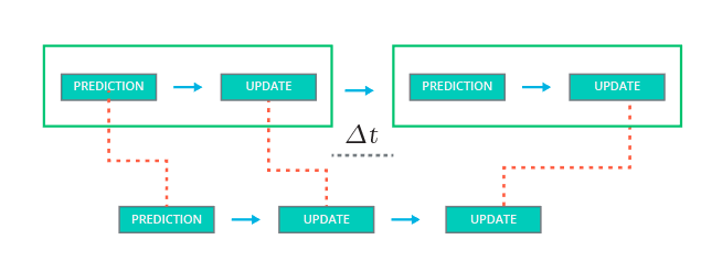
- 해당 Class는 칼만필터의
Init(VectorXd &x_in, MatrixXd &P_in, MatrixXd &F_in, MatrixXd &H_in, MatrixXd &R_in, MatrixXd &Q_in)- 해당 함수에서 Lidar냐 Radar냐에 따라 H, R 매트릭스를 교체해 주는 역할을 수행한다.
- 물론, 초기화 단계에서 칼만시스템의 매트릭스를 초기화해주는 역할도 수행한다.
Predict()- 아래 코드와 같이 total probability 이론에 따라 불확실성이 더해짐과 동시에 예측값을 출력한다.
x_ = F_ * x_ + u;
P_ = F_ * P_ * F_.transpose() + Q_;
- 아래 코드와 같이 total probability 이론에 따라 불확실성이 더해짐과 동시에 예측값을 출력한다.
Update(const VectorXd &z)- Lidar 데이터가 들어오는 경우, 수신되는 데이터가
state와 동일하게 cartesian coordinates를 따르는{px, py}가 수신되므로 Extended 접근을 할 필요가 없다. - 따라서, 아래의 칼만 시스템의
update수식에 맞게끔 보정을 수행한다.std::cout << "Lidar Update: \n"; VectorXd y = z - H_ * x_; MatrixXd S = H_ * P_ * H_.transpose() + R_; MatrixXd K = P_ * H_.transpose() * S.inverse(); x_ = x_ + K*y; P_ = P_ - K*H_*P_;
- Lidar 데이터가 들어오는 경우, 수신되는 데이터가
UpdateEKF(const VectorXd &z)- Radar 데이터가 들어오는 경우, 수신되는 데이터가
state의 cartesian coordinates랑 다른 polar coordinates의{rho, theta, dot_rho}가 들어오므로 이에 따른 비선형성이 발생한다. - 비선형성을 해소하기 위해 현재 state를 기준으로 1차 jacobian 선형화를 수행하여 칼만 시스템을 적용한 것이 Extended Kalman Filter이다.
- 따라서, H 매트릭스는 jacobian 선형화를 수행한 값을 대입해주었다.
- 선형화된 H 매트릭스는
4-2에서도 언급한 바와 같이 칼만 공분산과 게인을 구할때만 사용하고 나머지에는 비선형 함수h(x)를 그대로 사용하는 것을 유념하길 바란다.- Extended Kalman Filter Equations
Although the mathematical proof is somewhat complex, it turns out that the Kalman filter equations and extended Kalman filter equations are very similar. The main differences are:
- the F matrix will be replaced by $F_j$ when calculating
P'. - the H matrix in the Kalman filter will be replaced by the
Jacobianmatrix $H_j$ when calculatingS, K, and P. - to calculate
x', the prediction update function, $f$, is used instead of the F matrix. - to calculate
y, the $h$ function is used instead of the H matrix. - One important point to reiterate is that the equation $y = z - Hx’$ for the Kalman filter does not become $y = z - H_jx$ for the extended Kalman filter. Instead, for extended Kalman filters, we’ll use the $h$ function directly to map predicted locations $x’$ from Cartesian to polar coordinates.
- the F matrix will be replaced by $F_j$ when calculating
- Extended Kalman Filter Equations
Although the mathematical proof is somewhat complex, it turns out that the Kalman filter equations and extended Kalman filter equations are very similar. The main differences are:
-
따라서, 에러 term인
VectorXd y = z - H*x가 아닌VectorXd y = z - z_pred를 사용하였고, z_pred 는h(x)이다. - 추가적으로 에러 term
y는 -PI~PI안에 위치 시키기 위해 아래와 같이 처리해주었다.if (y(1) < -M_PI) y(1) += 2*M_PI; else if (y(1) > M_PI) y(1) -= 2*M_PI; - 칼만게인을 구하고 보정하고, 공분산을 업데이트하는것은 선형 칼만필터와 동일하다.
- 본 프로젝트에서는 H매트릭스를 선형화해서 사용하였다. (It is called EKF)
- Radar 데이터가 들어오는 경우, 수신되는 데이터가
- 개요:
4. Conclusion
- 데이터(Simulator)에서 dt(Sampling Time)를 찾아 헤맨 부분이 있었다. 설명이 나와 있지 않아 다른 코드를 참고해보니,
(time_stamp - previouse_time_stamp)/1000000.0해주었길래 같게 하니 잘 작동하였다. - Process Covariance
Q는 Hyper Parameter라고만 생각했는데, 경우에 따라 센서 NOISE SPEC만 정확히 주어진다면 Q자체도 수식으로 계산될 수 있음을 알게되었다. Lecture 10 of Lesson 24. - 본 프로젝트에서는 동일 object에 대한 tracking은 없이, 동일/싱글 타겟이 지속적으로 수신되는 것을 가정하고 진행하였으나, 실제 센서는 여러 object에 대한 데이터를 출력하므로 Tracking 알고리즘이 필요하다. (`Nearest Neighborhood, Simularity Score, PDA 등’)
끝
